Introducción a la planificación de la demanda
Conocer cómo es la demanda, cuáles son las características, las necesidades, los comportamientos, los deseos y las actitudes de los clientes, resulta una cuestión de alta importancia para las compañías ya sea manufactureras, distribuidores o minoristas para facilitar la planificación, gestión de inventarios, asignación de personal y todo lo que involucra la gestión en la cadena de suministros.
En el entorno actual del mercado, la
volatilidad de la demanda, la cada vez menor fidelidad de los clientes, los
ciclos de producto cada vez más cortos y la dura competencia global, son
elementos cuya presencia es incuestionable. Las empresas necesitan, cada vez más,
información que les permita tomar decisiones correctas, en tiempo real, que
aseguren la satisfacción de sus clientes como su primera prioridad, a la vez
que se mantienen competitivas y protegen sus márgenes comerciales.
Errores en las previsiones de la demanda, cuando
es en ésta en la que se basa la compra de materiales y la planificación de la
capacidad de producción, generan no solo inventaros en exceso, si no también clientes
insatisfechos a los que no podemos servir. Los fabricantes están cada vez más
utilizando técnicas más sofisticadas de planificación, con las que desarrollan
sus planes de producción en respuesta a cambios súbitos de la demanda. Los datos
que se manejan no solo vienen de las propias organizaciones, sino que muchas
veces vienen de proveedores, agentes distribuidores e incluso de los propios
clientes.
El pronóstico de la demanda desempeña un papel muy importante en la Gestión de la Cadena de Suministro. Obtener los pronósticos de demanda en la cadena de suministro puede ayudar a los expertos que toman las decisiones de cálculos de costos de producción y de materia prima, así como determinar los precios de ventas. Esto tiene como resultado niveles más bajos de inventario y lograr el JIT.

Objetivos
Los objetivos de este curso son:
1. Conocer los conceptos básicos de la planificación de demanda.
2. Aplicar las herramientas para la planificación de demanda.
Asignación 1
1. Conocer los conceptos básicos de la planificación de demanda.
2. Aplicar las herramientas para la planificación de demanda.
Asignación 1
Asignaciones para la planificación de demanda
La primera asignación es ver el video del IIT sobre el pronóstico
Asignación 2
Asignación 2
Lectura del libro Principles of Forecasting
La siguiente actividad es la lectura del libro Principles of Forecasting de Jon Scott Armstrong
Recursos
En esta sección veran un listado de bibliografia auxiliar para el desarrollo del curso
Supply chain
From Wikipedia, the free encyclopedia
A supply chain is actually a complex and dynamic supply and demand network.[1] (cf. Wieland/Wallenburg, 2011)
Contents |
Overview
The Council of Supply Chain Management Professionals (CSCMP) defines Supply Chain Management as follows: “Supply Chain Management encompasses the planning and management of all activities involved in sourcing and procurement, conversion, and all logistics management activities. Importantly, it also includes coordination and collaboration with channel partners, which can be suppliers, intermediaries, third-party service providers, and customers. In essence, supply chain management integrates supply and demand management within and across companies. Supply Chain Management is an integrating function with primary responsibility for linking major business functions and business processes within and across companies into a cohesive and high-performing business model. It includes all of the logistics management activities noted above, as well as manufacturing operations, and it drives coordination of processes and activities with and across marketing, sales, product design, finance and information technology.”
A typical supply chain begins with ecological and biological regulation of natural resources, followed by the human extraction of raw material, and includes several production links (e.g., component construction, assembly, and merging) before moving on to several layers of storage facilities of ever-decreasing size and ever more remote geographical locations, and finally reaching the consumer.
Many of the exchanges encountered in the supply chain will therefore be between different companies that will seek to maximize their revenue within their sphere of interest, but may have little or no knowledge or interest in the remaining players in the supply chain. More recently, the loosely coupled, self-organizing network of businesses that cooperates to provide product and service offerings has been called the Extended Enterprise.[citation needed]Supply chain modeling
A diagram of a supply chain. The black arrow represents the flow of materials and information and the gray arrow represents the flow of information and backhauls. The elements are (a) the initial supplier, (b) a supplier, (c) a manufacturer (production), (d) a customer, (e) the final customer.
There are a variety of supply chain models, which address both the upstream and downstream sides. However the SCOR model is most common.
The SCOR Supply-Chain Operations Reference model, developed by the Supply Chain Council, measures total supply chain performance. It is a process reference model for supply-chain management, spanning from the supplier's supplier to the customer's customer.[3] It includes delivery and order fulfillment performance, production flexibility, warranty and returns processing costs, inventory and asset turns, and other factors in evaluating the overall effective performance of a supply chain.The Global Supply Chain Forum (GSCF) introduced another Supply Chain Model. This framework[4] is built on eight key business processes that are both cross-functional and cross-firm in nature. Each process is managed by a cross-functional team, including representatives from logistics, production, purchasing, finance, marketing and research and development. While each process will interface with key customers and suppliers, the customer relationship management and supplier relationship management processes form the critical linkages in the supply chain.
The American Productivity & Quality Center (APQC) Process Classification Framework (PCF) SM is a high-level, industry-neutral enterprise process model that allows organizations to see their business processes from a cross-industry viewpoint. The PCF was developed by APQC and its member companies as an open standard to facilitate improvement through process management and benchmarking, regardless of industry, size, or geography. The PCF organizes operating and management processes into 12 enterprise level categories, including process groups, and over 1,000 processes and associated activities.
Supply chain management
A German paper factory receives its daily supply of 75 tons of recyclable paper as its raw material In the 1980s, the term Supply Chain Management (SCM) was developed[5] to express the need to integrate the key business processes, from end user through original suppliers. Original suppliers being those that provide products, services and information that add value for customers and other stakeholders. The basic idea behind the SCM is that companies and corporations involve themselves in a supply chain by exchanging information regarding market fluctuations and production capabilities.
If all relevant information is accessible to any relevant company, every company in the supply chain has the possibility to and can seek to help optimizing the entire supply chain rather than sub optimize based on a local interest. This will lead to better planned overall production and distribution which can cut costs and give a more attractive final product leading to better sales and better overall results for the companies involved.Incorporating SCM successfully leads to a new kind of competition on the global market where competition is no longer of the company versus company form but rather takes on a supply chain versus supply chain form.
There is often confusion over the terms supply chain and logistics. It is now generally accepted that the term Logistics applies to activities within one company/organization involving distribution of product whereas the term supply chain also encompasses manufacturing and procurement and therefore has a much broader focus as it involves multiple enterprises, including suppliers, manufacturers and retailers, working together to meet a customer need for a product or service.[citation needed]
Starting in the 1990s several companies chose to outsource the logistics aspect of supply chain management by partnering with a 3PL, Third-party logistics provider. Companies also outsource production to contract manufacturers.[6] Technology companies have risen to meet the demand to help manage these complex systems.
There are actually four common Supply Chain Models. Besides the two mentioned above, there are the American Productivity & Quality Center's (APQC) Process Classification Framework and the Supply Chain Best Practices Framework
An unusual food supply chain operated by Dabbawalas in Mumbai is noted for being extremely reliable without using any computers or modern technology. It has been verified to be a six sigma supply chain.[7]
Regulations
Supply chain security has become particularly important in recent years. As a result, supply chains are often subject to global and local regulations. Several major regulations emerged in 2010 alone that have had a lasting impact on how global supply chains operate. These new regulations include: The Importer Security Filing (ISF)[8] additional provisions of the Certified Cargo Screening Program (CCSP) [9].Development and design
With increasing globalization and easier access to alternative products in today’s markets, the importance of product design in demand generation is more significant than ever. In addition, as supply, and therefore competition, among companies for the limited market demand increases and pricing and other marketing elements become less distinguishing factors, product design also plays a different role by providing attractive features to generate demand. In this context, demand generation is used to define how attractive a product design is in terms of creating demand.In other words, it is the ability of a product design to generate demand by satisfying customer expectations. However, product design impacts not only demand generation, but also manufacturing processes, cost, quality, and lead time. The product design affects the associated supply chain and its requirements directly including, but not limited to: manufacturing, transportation, quality, quantity, production schedule, material selection, production technologies, production policies, regulations, and laws. From a broad perspective, the success of the supply chain depends on the product design and the capabilities of the supply chain, but the reverse is also true—the success of the product depends on the supply chain that produces it.
Since the product design dictates multiple requirements on the supply chain, as mentioned previously, it is clear that once a product design is completed, it drives the structure of the supply chain, limiting the flexibility of the engineers to generate and evaluate different (potentially more cost effective) supply chain alternatives.[10]
See also
- American Production and Inventory Control Society
- Chemicals, Tire, and Process Industries (CTP)
- Cold chain
- Council of Supply Chain Management Professionals
- Demand chain
- Demand chain management
- Demand optimization
- Document automation in supply chain management & logistics
- Distribution
- Distribution resource planning
- Factory Physics
- Extended Enterprise
- Industrial engineering
- Inventory control
- Last mile (transportation)
- Liquid logistics
- Logistics
- Military supply chain management
- Nomenclature
- Reverse logistics
- Supply network
- Supply chain management
- Supply chain network
- Supply-Chain Operations Reference Model
- Supply chain optimization
- Supply Chain Risk Management
- Supply chain security
- Value chain
- Value network
- Vertical integration
References
- ^ cf. Andreas Wieland, Carl Marcus Wallenburg (2011): Supply-Chain-Management in stürmischen Zeiten. Berlin.
- ^ Anna Nagurney: Supply Chain Network Economics: Dynamics of Prices, Flows, and Profits, Edward Elgar Publishing, 2006, ISBN 1-84542-916-8
- ^ SCC Supply Chain Council, SCOR Model
- ^ the Supply Chain Management Institute - framework
- ^ Oliver, R.K., Webber, M.D., 1982, “Supply-chain management: logistics catches up with strategy”, Outlook, Booz, Allen and Hamilton Inc. Reprinted 1992, in Logistics: The Strategic Issues, ed. M Christopher, Chapman Hall, London, pp. 63-75.
- ^ Selecting a Third Party Logistics (3PL) Provider Martin Murray, about.com
- ^ [1]
- ^ http://www.cbp.gov/linkhandler/cgov/newsroom/publications/trade/import_sf_carry.ctt/import_sf_carry.pdf
- ^ http://www.tsa.gov/what_we_do/layers/aircargo/certified_screening.shtm
- ^ Gokhan, Nuri Mehmet; Needy, Norman (December 2010). "Development of a Simultaneous Design for Supply Chain Process for the Optimization of the Product Design and Supply Chain Configuration Problem.". Engineering Management Journal 22 (4): 20–30.
External links
| Look up supply chain in Wiktionary, the free dictionary. |
| Wikimedia Commons has media related to: Supply chain |
Este artículo es licenciado bajo la licenciaLicencia GNU. Usa material deArtículo"Supply chain".
FORECAST (model)
From Wikipedia, the free encyclopedia
(Redirected from Forecast model)
FORECAST is a management-oriented, stand-level, forest-growth and ecosystem-dynamics model. The model was designed to accommodate a wide variety of silvicultural and harvesting systems and natural disturbance events (e.g., fire, wind, insect epidemics) in order to compare and contrast their effect on forest productivity, stand dynamics, and a series of biophysical indicators of non-timber values.
Contents |
Model description
Projection of stand growth and ecosystem dynamics is based upon a representation of the rates of key ecological processes regulating the availability of, and competition for, light and nutrient resources (a representation of moisture effects on soil processes, plant physiology and growth, and the consequences of moisture competition is being added). The rates of these processes are calculated from a combination of historical bioassay data (such as biomass accumulation in plant components and changes in stand density over time) and measures of certain ecosystem variables (including decomposition rates, photosynthetic saturation curves, and plant tissue nutrient concentrations) by relating ‘biologically active’ biomass components (foliage and small roots) to calculated values of nutrient uptake, the capture of light energy, and net primary production. Using this ‘internal calibration’ or hybrid approach, the model generates a suite of growth properties for each tree and understory plant species that is to be represented in a subsequent simulation. These growth properties are used to model growth as a function of resource availability and competition. They include (but are not limited to): (1) photosynthetic efficiency per unit foliage biomass and its nitrogen content based on relationships between foliage nitrogen, simulated self-shading, and net primary productivity after accounting for litterfall and mortality; (2) nutrient uptake requirements based on rates of biomass accumulation and literature- or field-based measures of nutrient concentrations in different biomass components on sites of different nutritional quality (i.e. fertility); (3) light-related measures of tree and branch mortality derived from stand density and live canopy height input data in combination with simulated vertical light profiles. Light levels at which mortality of branches and individual trees occur are estimated for each species.[1] Many of FORECAST’s calculations are made at the stand level, but the model includes a sub-model which disaggregates stand-level productivity into the growth of individual stems with user-supplied information on stem size distributions at different stand ages. Top height and DBH are calculated for each stem and used in a taper function to calculate total and individual gross and merchantable volumes. Snags and logs are created in the model from natural stand self-thinning (mainly due to light competition) and from different types of user-defined disturbance events such as insect/disease-induced mortality, windthrow, non-commercial thinning and stand harvesting. Snag fall rates and log-decomposition are simulated using species-specific and tree-size-specific decay parameters derived from the literature, expert opinion, or field measurements.[1]The process of model application
FORECAST has four stages in its application: 1) data assembly and input verification, 2) establishing the ecosystem condition for the beginning of a simulation run (by simulating the known or assumed history of the site), 3) defining a management and/or natural disturbance regime, and 4) simulating this regime and analyzing model output. The first two stages represent model calibration. Calibration data are assembled that describe the accumulation of biomass (above and below-ground components) in trees and minor vegetation for three chronosequences of stands, each one developed under relatively homogeneous site conditions, representing three different nutritional site qualities. Tree biomass and stand self-thinning rate data are often generated from the height, DBH and stand density output of traditional growth and yield models in conjunction with species-specific component biomass allometric equations. To calibrate the nutritional aspects of the model, data describing the concentration of nutrients in the various biomass components are required. FORECAST also requires data on the degree of shading produced by different quantities of foliage and the photosynthetic response of foliage to different light levels (photosynthetic light saturation curves for either average foliage or separately for sun and shade adapted foliage). A comparable but simpler set of data for minor vegetation must be provided if the user wishes to represent this ecosystem component. Lastly, data describing the rates of decomposition of various litter types and soil organic matter are required for the model to simulate nutrient cycling. Simulation of soil leaching losses and certain measures of soil nutrient availability require input data that define cation and anion exchange capacity data for organic matter and mineral soil, and sorption-desorption processes. The second aspect of calibration requires running the model in “set-up” mode to establish initial site conditions. The detailed representation of many different litter types and soil organic matter conditions makes it impractical to measure initial litter and soil pools and conditions directly in the field; consequently, the model is used to generate starting conditions.[2]Complexity of the model
As an ecosystem level model FORECAST offers the user the ability to represent a high degree of complexity in vegetation (multiple species and different life forms), plant community structure (canopy layering as a simple even-age single canopy layer or a complex multi-age, multi canopy) and population, community and ecosystem processes. However, the model can be simplified to any desired level of complexity that matches the user’s interests, specific application and data availability. In its simplest form it can be run as a single age cohort, plant monoculture, light competition model. At the other extreme the model can be used to simulate succession and disturbance responses in a complex multi species, multi age cohort ecosystem-level application with population, community and ecosystem processes represented with light, nutrient and moisture effects and their interactions, and the possibility to examine potential climate change effects.Model extensions and linkages
FORECAST has been extended to a spatially-explicit landscape local level (LLEMS)[3], a spatially-explicit individual tree model FORCEE, and to an interactive 3-D visualization (CALP Forester), FORECAST has been linked to a variety of landscape-level models such as ATLAS and DYNA-PLAN.[4] The model has been used as the foundation for two educational applications (FORTOON and POSSIBLE FOREST FUTURES)[5]Model evaluation
FORECAST has been validated against field data for a range of growth and yield and structural variables in: coastal Western Hemlock zone in British Columbia [6], coastal Douglas-fir forests,[2] [7] and interior mixedwood forests in British Columbia[8][6]History of model application
FORECAST model has been applied to a variety of forest types: mixed Douglas-fir and paper birch forest [9], mixed aspen and white spruce forest [10] [11], Chinese-fir plantations [12], coastal Douglas-fir forest.[2]External links
- Official website of the model
- Model evaluation for coastal British Columbia and example of model application for simulation of variable retention harvest and projection of recovery of old-growth structural attributes
- Model evaluation
- Model application for forest management
- Simulation of carbon balance using the FORECAST model
- Model description on the forest-growth models list
References
- ^ a b Kimmins, J.P.; D. Mailly, b. Seely (20 October 1999). "Modelling forest ecosystem net primary production: the hybrid simulation approach used in FORECAST". Ecological Modelling (Elsevier Science B.V.) 122 (3): 195–224. doi:10.1016/S0304-3800(99)00138-6.
- ^ a b c Blanco, J.A.; Seely, B., Welham, C., Kimmins, J.P. & Seebacher, T.M. (1 October 2008). "Testing the performance of a forest ecosystem model (FORECAST) against 29 years of field data in a Pseudotsuga menziesii plantation". Canadian Journal of Forest Research (NRC Research Press) 37 (10): 1808–1820.
- ^ http://www.forrex.org/program/forest/ESD/PDF/Workshops/Science_Forum/Seely.pdf
- ^ "The Models: Summary of Model Linkages and Integration for K2". Kamloops Future Forest Strategy II. http://k2kamloopstsa.com/the-models/. Retrieved December 2, 2010.
- ^ http://www.forrex.org/events/mountainpinebeetleforum/PDF/UBC/Hamish%20Kimmins.pdf
- ^ a b Gerzon, Michael (2005). Modelling the Recovery of Old-Growth Attributes in Coastal Western Hemlock Forests Following Management and Natural Disturbances (M.S. thesis). University of British Columbia. http://www.forestry.ubc.ca/ecomodels/team/thesis/Gerzon%202009%20thesis.pdf. Retrieved December 2, 2010.
- ^ Boldor, Marius Ioan (2007). A Field and Simulation Study of the Initiation Phase in Douglas-Fir Plantations (M.S. thesis). University of British Columbia. http://www.forestry.ubc.ca/ecomodels/team/thesis/Boldor%202007%20thesis.pdf. Retrieved December 2, 2010.
- ^ Seely, B.; Hawkins C., Blanco J.A., Welham C., Kimmins J.P. (August 2009). "Evaluation of an ecosystem-based approach to mixedwood modelling". Forest Growth and Timber Quality: Crown Models and Simulation Methods for Sustainable Forest Management. Portland, OR: United States Forest Service (General Technical Report PNW-GTR-791). pp. 205-210. http://citeseerx.ist.psu.edu/viewdoc/download?doi=10.1.1.150.4159&rep=rep1&type=pdf#page=217. Retrieved December 2, 2010.
- ^ Sachs, D. (1996). Simulation of the growth of mixed stands of Douglas-fir and paper birch using the FORECAST model. Silviculture of temperate and boreal broadleaf conifer mixtures (eds P.G. Comeau & K.D. Thomas), pp. 152. BC Ministry of Forests, Victoria, BC, Canada.
- ^ Welham, C., B. Seely and J.P. Kimmins. 2002. The utility of the two-pass harvesting system: an analysis using the ecosystem simulation model FORECAST. Can. J. For. Res. 32:1071-1079.
- ^ Seely, B.; Welham, C., Kimmins, H. (15 September 2002). "Carbon sequestration in a boreal forest ecosystem: results from the ecosystem simulation model, FORECAST". Forest Ecology and Management (Elsevier Science B.V.) 169 (1-2): 123–135. doi:10.1016/S0378-1127(02)00303-1.
- ^ Bi J., Blanco J.A., Kimmins J.P., Ding Y., Seely B., Welham C. 2007. Yield decline in Chinese Fir plantations: A simulation investigation with implications for model complexity. Can. J. For. Res. 37: 1615-1630.
Este artículo es licenciado bajo la licenciaLicencia GNU. Usa material deArtículo"Forecast model".
Evaluación
Caso de estudio
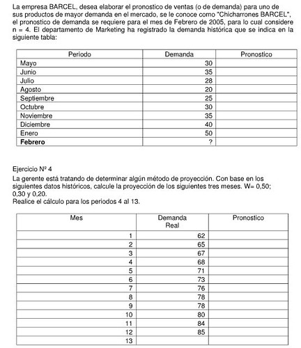
En esta sección se presentan dos problemas relacionados con las proyecciones de demandas.
¿Cual es el costo de malos pronósticos?
Tenemos garantía que los pronósticos no van a ser 100% exactos y que ademas la desviación de los pronósticos tiene un costo implícito, ya sea que los pronósticos fueron altos o bajos respecto a la realidad. el punto fundamental en los pronósticos es ser consientes y lograr la menor desviación respecto a los objetivos:
1. Pronosticar por arriba de la demanda tiene entre sus consecuencias exceso de inventario, obsolenscencia, reducción de margen para promover su venta.
2. Pronosticar por debajo de la demanda tiene ente sus consecuencias comprar y producir más caro algo que no estaba planeado, incluso pérdida de venta y margen si no reaccionamos a tiempo.
No hay comentarios:
Publicar un comentario